Porosity Maps

This page documents the continuum porosity-map workflow implemented in voids.image.porosity. It is separate from pore-network porosity: here the output is a regular grid of cell-average porosity values intended for continuum, FEM, finite-volume, or external solver workflows.

The minimal demonstration is notebooks/33_mwe_synthetic_porosity_maps, which builds porosity maps from a synthetic PoreSpy blobs binary image and a derived toy grayscale image.

---

What block_shape Means

block_shape defines how many fine image voxels are averaged into one porosity-map cell.

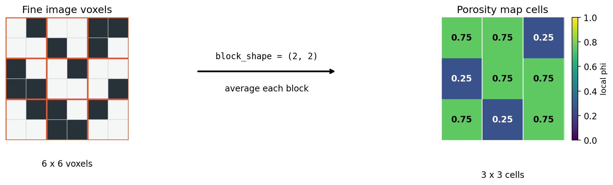
The 2-D schematic shows the same operation used in 3-D: each highlighted fine voxel block becomes one coarse cell whose value is the average porosity over that block.

For a 3-D image with shape

\[ (n_0, n_1, n_2), \]

and coarse-cell block sizes \((b_0, b_1, b_2)\), represented in code by block_shape=(b_0, b_1, b_2),

the output porosity map has shape

\[ \left( \left\lfloor \frac{n_0}{b_0} \right\rfloor, \left\lfloor \frac{n_1}{b_1} \right\rfloor, \left\lfloor \frac{n_2}{b_2} \right\rfloor \right). \]

When strict=True, which is the default, every image dimension must be exactly divisible by the corresponding block dimension. For example:

shape = (300, 300, 300)
block_shape = (10, 10, 10)

gives a porosity map with shape:

\[ (30, 30, 30). \]

Each coarse porosity cell is the average over one \(10 \times 10 \times 10\) voxel block. If the fine voxel size is \(40\,\mu\mathrm{m}\), then the porosity-map cell size is:

\[ (10, 10, 10) \times 40\,\mu\mathrm{m} = (400, 400, 400)\,\mu\mathrm{m}. \]

In code:

porosity = porosity_map_from_binary(
    image,
    block_shape=(10, 10, 10),
    voxel_size=40.0e-6,
)

porosity.shape       # (30, 30, 30)
porosity.cell_size   # (4.0e-4, 4.0e-4, 4.0e-4) in meters

Axis convention

block_shape follows the NumPy array axis order of the input image. voids does not silently reinterpret array axes as geological or scanner axes. If a dataset uses a different physical axis order, transpose or document that convention before exporting fields to another solver.

---

Binary-Image Porosity

For a segmented binary image, the input is interpreted as a void mask. By default:

• True or 1 means void,
• False or 0 means solid.

Let \(V_{ijk}\) be the fine-grid void indicator:

\[ V_{ijk} = \begin{cases} 1, & \text{if voxel }(i,j,k)\text{ is void}, \\ 0, & \text{if voxel }(i,j,k)\text{ is solid}. \end{cases} \]

For porosity-map cell \((I,J,K)\), with block shape \((b_0,b_1,b_2)\), the local porosity is:

\[ \phi^{\mathrm{bin}}_{IJK} = \frac{1}{b_0 b_1 b_2} \sum_{i=I b_0}^{(I+1)b_0 - 1} \sum_{j=J b_1}^{(J+1)b_1 - 1} \sum_{k=K b_2}^{(K+1)b_2 - 1} V_{ijk}. \]

So the binary porosity map is exactly a local void-volume fraction on the regular image grid.

If image_is_void=False, the input binary image is interpreted as a solid mask and inverted before applying the same formula.

Conservation Check

If the image shape is exactly divisible by block_shape, the mean of the local porosity map equals the global void fraction:

\[ \overline{\phi}^{\mathrm{bin}} = \frac{1}{N_c}\sum_{IJK}\phi^{\mathrm{bin}}_{IJK} = \frac{1}{N_v}\sum_{ijk}V_{ijk}, \]

where \(N_c\) is the number of coarse cells and \(N_v\) is the number of fine voxels.

This is one of the most important synthetic verification checks.

---

Grayscale-Image Porosity

For a grayscale image, voids first maps each fine voxel intensity to a porosity value using a two-point linear calibration.

The calibration inputs are:

Parameter	Meaning
solid_gray	grayscale value assigned to background_porosity
pore_gray	grayscale value assigned to porosity \(1\)
background_porosity	porosity floor at the solid endpoint

Let \(G_{ijk}\) be the grayscale value of voxel \((i,j,k)\), \(G_s\) be solid_gray, \(G_p\) be pore_gray, and \(\phi_b\) be background_porosity. The voxel-scale porosity is:

\[ \phi^{\mathrm{vox}}_{ijk} = \phi_b + (1-\phi_b) \frac{G_{ijk} - G_s}{G_p - G_s}. \]

By default, values are clipped to:

\[ \phi^{\mathrm{vox}}_{ijk} \in [\phi_b, 1]. \]

Then the coarse grayscale porosity map is a block average of those voxel porosities:

\[ \phi^{\mathrm{gray}}_{IJK} = \frac{1}{b_0 b_1 b_2} \sum_{i=I b_0}^{(I+1)b_0 - 1} \sum_{j=J b_1}^{(J+1)b_1 - 1} \sum_{k=K b_2}^{(K+1)b_2 - 1} \phi^{\mathrm{vox}}_{ijk}. \]

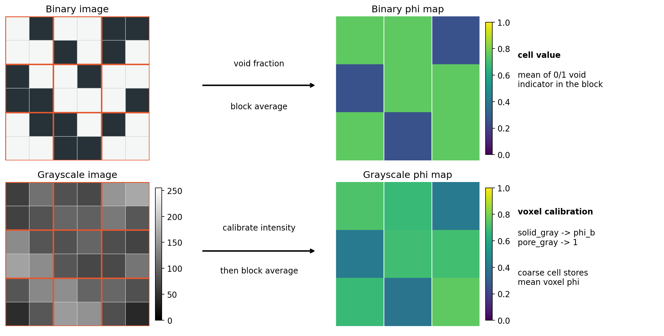
The top row corresponds to the binary void-fraction formula. The bottom row corresponds to the grayscale calibration formula followed by the same block average.

Micro-CT Grayscale Calibration In The Literature

Ferreira et al. (2020) used resampled micro-CT images of carbonate plugs to construct porosity fields for a two-scale continuum reactive-flow solver. The image-to-porosity calculation assigns a pore grayscale threshold to 100% porosity, a solid grayscale threshold to a background porosity \(BP\), and linearly maps each micro-CT voxel between those endpoints. In fractional notation, the same calculation is:

\[ \epsilon_{\mathrm{voxel}} = BP + (1-BP) \frac{GS_{\mathrm{voxel}}-GS_{\mathrm{solid}}} {GS_{\mathrm{pore}}-GS_{\mathrm{solid}}}. \]

This is the same two-endpoint linear calibration implemented by calibrated_porosity_from_grayscale, with background_porosity playing the role of \(BP\). The additional block_shape averaging in voids is a separate coarsening step: use block_shape=(1, 1, 1) when each image voxel is intended to become one continuum cell, or use larger blocks when the target solver uses a coarser regular grid.

Dark-Pore And Bright-Pore Images

The formula does not require pores to be darker than solid. It only requires solid_gray and pore_gray to be distinct.

For a dark-pore image:

\[ G_p < G_s. \]

For a bright-pore image:

\[ G_p > G_s. \]

Both cases are handled by the same denominator \(G_p - G_s\).

Important Assumption

The grayscale path assumes that a linear grayscale interpolation is a defensible proxy for local porosity between the two calibration endpoints. That may be incorrect when the image has severe beam hardening, ring artifacts, mixed mineral phases, uncorrected scanner drift, or a nonlinear intensity-density relationship. For real micro-CT data, calibration must be treated as part of the physical model, not as a plotting choice.

---

Physical Volumes

For a porosity map with cell size

\[ (\Delta x, \Delta y, \Delta z), \]

the bulk volume of one porosity cell is:

\[ \Delta V = \Delta x \Delta y \Delta z. \]

The total represented bulk volume is:

\[ V_{\mathrm{bulk}} = N_c \Delta V. \]

The implied pore volume is:

\[ V_{\mathrm{void}} = \sum_{IJK}\phi_{IJK}\Delta V. \]

The mean porosity is therefore:

\[ \overline{\phi} = \frac{V_{\mathrm{void}}}{V_{\mathrm{bulk}}}. \]

This relation is used by PorosityMap.bulk_volume, PorosityMap.void_volume, and PorosityMap.mean_porosity.

2-D maps

The same implementation accepts 2-D arrays, where the product of cell_size is an area. If the target solver expects a 3-D volume, supply a 3-D image or define an explicit thickness outside this 2-D helper.

---

Kozeny-Carman Permeability Field

voids can also generate an associated permeability field from a porosity map using the Kozeny-Carman closure. For cell porosity \(\phi\), characteristic length \(d\), and Kozeny constant \(C\), the implemented permeability form is:

\[ k(\phi) = \frac{d^2 \phi^3}{C(1-\phi)^2}, \quad 0 < \phi < 1. \]

The equivalent inverse-permeability, or Darcy resistance, form is:

\[ k^{-1}(\phi) = \frac{C(1-\phi)^2}{d^2\phi^3}, \quad 0 < \phi < 1. \]

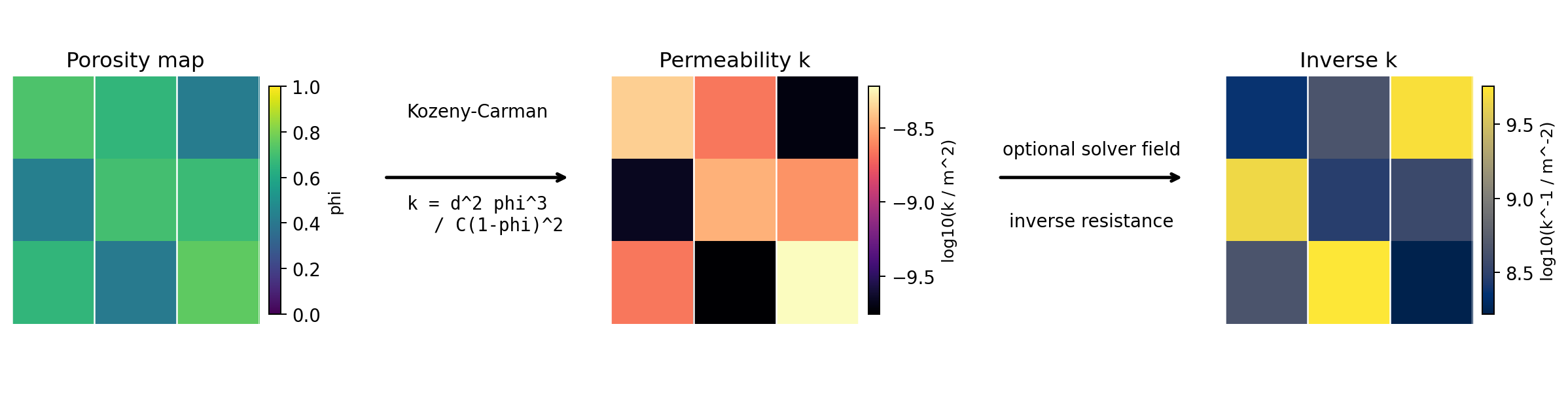
The permeability map and inverse-permeability map live on the same regular grid as the porosity map. The figure uses a logarithmic color scale for \(k\) and \(k^{-1}\), because permeability closures can vary by orders of magnitude.

The default \(C=180\) is the common packed-sphere Kozeny-Carman value associated with the classical Kozeny and Carman packed-bed relation. The length \(d\) is a model parameter, not inferred automatically. In a sub-resolution porosity interpretation, \(d\) is often tied to the voxel or control-volume length scale when no better grain-scale or micropore-scale calibration is available, but that choice is empirical and should be tested.

The endpoint limits are:

\[ \phi=0 \Rightarrow k=0,\quad k^{-1}=\infty, \]

\[ \phi=1 \Rightarrow k=\infty,\quad k^{-1}=0. \]

These are mathematical limits. Many external solvers require finite values, so voids exposes explicit caps and endpoint parameters:

from voids.image.porosity import permeability_map_from_porosity

permeability = permeability_map_from_porosity(
    porosity,
    characteristic_length=4.0e-4,
    kozeny_constant=180.0,
    max_permeability=1.0e-8,
)

The resulting object is a PermeabilityMap on the same grid as the input porosity map:

permeability.values          # k field
permeability.inverse_values  # k^{-1} field for Darcy-Brinkman resistance terms
permeability.cell_size       # inherited from the porosity map

Closure calibration

The Kozeny-Carman field is a closure model, not a direct measurement. The same porosity map can produce very different permeability fields if \(d\), \(C\), endpoint handling, or caps are changed. For real data, these parameters should be calibrated or at least sensitivity-tested against laboratory permeability, direct numerical simulation, or another reference.

---

Exported HDF5 Files

save_porosity_map_hdf5 writes:

• /porosity: the cell-average porosity array,
• root attribute schema_version,
• root attribute metadata, encoded as JSON.

save_permeability_map_hdf5 writes:

• /permeability: the cell-wise permeability array,
• root attribute schema_version,
• root attribute metadata, encoded as JSON.

The metadata includes:

• porosity-map shape,
• cell size,
• origin,
• units,
• source/calibration metadata such as block_shape, solid_gray, pore_gray, and background_porosity.

This export is intentionally solver-neutral. It is a stable field file, not a full FEM mesh. Solver-specific exporters should define cell ordering, mesh topology, boundary patches, and field naming explicitly.

---

Structured Mesh Export

voids.mesh can convert a regular PorosityMap, optionally paired with a matching PermeabilityMap, into a structured mesh. The default cells are quadrilaterals for 2-D maps and hexahedra for 3-D maps. If a downstream solver expects simplex cells, the same map grid can also be subdivided into triangles in 2-D or tetrahedra in 3-D. The cell data order is explicit:

cell_data["porosity"][0][n] == porosity.values.ravel(order="C")[n]

This means the mesh is a representation of the coarse map grid, not a segmentation-boundary mesh of the original image. For a 2-D slice, each coarse porosity cell becomes one quadrilateral by default, or two triangles when element_type="triangle". For a 3-D map, each coarse porosity cell becomes one hexahedron by default, or six tetrahedra when element_type="tetra" or element_type="tetrahedron". In the simplex exports, the child cells inherit the same porosity, permeability, and parent cell_index values as the original coarse map cell.

The 2-D scheme shows the default cell-for-cell quadrilateral export. The 3-D default is analogous: each coarse map volume cell becomes one hexahedral mesh cell instead of one quadrilateral. The simplex options subdivide those default cells, but porosity and permeability remain cell-wise fields inherited from the parent map cell.

from voids.mesh import write_structured_map_meshes

paths = write_structured_map_meshes(
    porosity,
    "outputs/case_a",
    stem="case_a_porosity_permeability",
    permeability_map=permeability,
    formats=("gmsh", "vtk", "vtu", "netgen"),
)

triangle_paths = write_structured_map_meshes(
    porosity,
    "outputs/case_a",
    stem="case_a_porosity_permeability_triangles",
    permeability_map=permeability,
    formats=("gmsh", "vtk", "vtu"),
    element_type="triangle",
)

The Gmsh .msh, VTK .vtk, and VTU .vtu exports are intended to carry the floating porosity and permeability arrays as cell data. The Netgen .vol writer available through meshio can write the structured geometry, but it should not be treated as the authoritative carrier of floating porosity/permeability fields. Keep the HDF5 map files, or a cell-data-preserving format such as VTU, as the source of truth for the coefficients.

voids uses meshio for mesh-file I/O. The meshio project documents support for Gmsh, VTK, VTU, Netgen, and many other formats, but format support does not imply that every downstream code preserves the same field-data names, physical tags, or boundary-region conventions. Check the exported mesh in the target solver before interpreting a simulation.

Gmsh export versus Gmsh meshing

The .msh export is a structured map mesh written in Gmsh format. It does not run Gmsh to remesh the bone/marrow interface. The triangular and tetrahedral options are structured subdivisions of the porosity-map cells, not boundary-conforming image-to-geometry meshes. If a later workflow needs a boundary-conforming triangular or tetrahedral mesh, the image-to-geometry step and boundary labels should be specified as a separate model.

---

Synthetic Verification Plan

Synthetic cases are useful because the expected porosity is known before running the code. They should be used before interpreting real scanner-derived fields.

1. All-Void And All-Solid Images

For an all-void binary image:

\[ V_{ijk}=1 \quad\Rightarrow\quad \phi_{IJK}=1 \quad\text{for all cells}. \]

For an all-solid binary image:

\[ V_{ijk}=0 \quad\Rightarrow\quad \phi_{IJK}=0 \quad\text{for all cells}. \]

These cases verify phase polarity and the averaging formula.

2. Known Block Fractions

Construct a small image where each block has a manually known number of void voxels. For example, a \(2 \times 2\) block with three void voxels must give:

\[ \phi = \frac{3}{4}. \]

This verifies that block_shape is applied in the expected axis order.

3. Global Conservation

For a binary image whose shape is divisible by block_shape, verify:

\[ \mathrm{mean}(\phi_{\mathrm{map}}) = \mathrm{mean}(V_{\mathrm{image}}). \]

This check is robust and should hold for random synthetic images, PoreSpy blobs, checkerboards, and hand-built masks.

4. Grayscale Endpoint Calibration

Use a tiny grayscale image containing only the calibration endpoints:

\[ G=G_p \Rightarrow \phi=1, \]

\[ G=G_s \Rightarrow \phi=\phi_b. \]

The midpoint should give:

\[ G=\frac{G_p+G_s}{2} \Rightarrow \phi=\phi_b+\frac{1-\phi_b}{2}. \]

This verifies the linear calibration independently of block averaging.

5. Binary-To-Grayscale Consistency

Generate a grayscale image directly from a binary image using exactly the two calibration endpoint intensities and no blur or noise:

\[ G_{ijk} = \begin{cases} G_p, & V_{ijk}=1,\\ G_s, & V_{ijk}=0. \end{cases} \]

If background_porosity=0, then:

\[ \phi^{\mathrm{gray}}_{IJK} = \phi^{\mathrm{bin}}_{IJK}. \]

If background_porosity > 0, then:

\[ \phi^{\mathrm{gray}}_{IJK} = \phi_b + (1-\phi_b)\phi^{\mathrm{bin}}_{IJK}. \]

This is the cleanest synthetic test connecting the binary and grayscale workflows.

6. HDF5 Round Trip

After export and import, verify:

\[ \phi_{\mathrm{loaded}} = \phi_{\mathrm{original}}, \]

and check that cell_size, origin, units, and calibration metadata are unchanged.

This verifies the interchange format, not the physical calibration.

7. Kozeny-Carman Closure Checks

For the permeability closure, verify the exact interior formula:

\[ k(\phi) = \frac{d^2 \phi^3}{C(1-\phi)^2}, \quad 0<\phi<1, \]

and the reciprocal relation:

\[ k(\phi)k^{-1}(\phi)=1. \]

Also verify endpoint behavior:

\[ \phi=0 \Rightarrow k=0, \]

\[ \phi=1 \Rightarrow k^{-1}=0. \]

If finite caps are supplied, verify that the cap is the only reason the output differs from the mathematical closure.

8. PoreSpy Blob Sanity Check

For a PoreSpy blobs realization with target porosity \(\phi_t\), check:

\[ \mathrm{mean}(V_{\mathrm{image}}) \approx \phi_t, \]

then check conservation:

\[ \mathrm{mean}(\phi_{\mathrm{map}}) = \mathrm{mean}(V_{\mathrm{image}}). \]

This verifies that the workflow preserves the realized synthetic image porosity. It does not prove that the morphology is realistic for a particular rock.

---

What This Does Not Validate

These calculations validate the mechanics of local porosity mapping. They do not, by themselves, validate:

• scanner grayscale calibration,
• beam-hardening correction,
• mineral-density interpretation,
• unresolved microporosity,
• permeability closure,
• connectivity or flow behavior,
• or agreement with laboratory porosity.

For real datasets, a defensible validation sequence should include:

1. record voxel size, image crop, support mask, and preprocessing,
2. document solid_gray, pore_gray, and background_porosity,
3. compare mean porosity against laboratory porosity or a trusted image-derived reference,
4. inspect slices of the grayscale image, binary segmentation, and porosity map,
5. test sensitivity to the calibration endpoints and block size,
6. only then export the field to an external continuum solver.

---

Relation To Published Micro-Continuum Models

The voids porosity-map representation is compatible with the micro-continuum porosity fields described by Soulaine and Tchelepi (2016) and Soulaine et al. (2016), but it does not implement their Darcy-Brinkman or Darcy-Brinkman-Stokes solver.

In Soulaine and Tchelepi (2016) and Soulaine et al. (2016), the central image-derived field is a local void fraction:

\[ \epsilon_f(\mathbf{x}) \in [0, 1], \]

and, specifically in the sub-resolution porosity formulation of Soulaine et al. (2016),

\[ \epsilon_{\mathrm{micro}}(\mathbf{x}) \in [0, 1]. \]

Cells with \(\epsilon_f=1\) represent fully resolved free-flow regions, cells with \(\epsilon_f=0\) represent solid or no-flow regions, and intermediate values represent porous control volumes whose sub-cell pore structure is not resolved. The flow model then uses a single-domain Darcy-Brinkman-type equation, with a permeability or inverse-permeability field coupled to porosity.

The voids porosity map stores the same type of mathematical object:

\[ \phi_{IJK} \in [0, 1], \]

a cell-average void fraction on a regular grid. Therefore, a PorosityMap.values array can be interpreted as a candidate \(\epsilon_f\) field for a micro-continuum solver if the control-volume size, axis order, and physical units are aligned with that solver.

The important difference is what voids currently does with the field.

Aspect	voids porosity map	Published micro-continuum model
Main field	Cell-average porosity \(\phi\)	Void fraction \(\epsilon_f\) or microporosity \(\epsilon_{\mathrm{micro}}\)
Binary image route	Block-average of a resolved void indicator	Compatible with a filtered control-volume porosity
Grayscale route	Linear grayscale-to-porosity calibration, then block average	Compatible only if calibration matches the image-processing assumptions
Flow equations	Not solved by this feature	Darcy-Brinkman or Darcy-Brinkman-Stokes single-domain solve
Permeability closure	Optional Kozeny-Carman \(k(\phi)\) and \(k^{-1}(\phi)\) field generation	Required, commonly specified as a porosity-dependent \(k=k(\epsilon)\) relation
Free-flow handling	Stored only as \(\phi=1\) cells	Solver switches toward Stokes/Navier-Stokes behavior
Porous/no-flow handling	Stored only as \(\phi=0\) or \(0<\phi<1\) cells	Solver gives high resistance or no flow depending on closure

Same Interpretation When block_shape=(1, 1, 1)

If the input image voxel is the intended micro-continuum control volume, then:

porosity = porosity_map_from_binary(
    image,
    block_shape=(1, 1, 1),
    voxel_size=voxel_size,
)

produces one porosity-map cell per image voxel. For a binary image, each value is either 0 or 1. For a calibrated grayscale image, each value can be intermediate and may be used as a sub-resolution porosity estimate.

This is closest to the voxel-wise porosity-field interpretation used in the sub-resolution porosity formulation of Soulaine et al. (2016).

Filtered Interpretation When block_shape > 1

When block_shape is larger than one, voids is not merely copying voxel labels. It is applying a spatial filter:

\[ \phi_{IJK} = \frac{1}{|B_{IJK}|} \sum_{(i,j,k)\in B_{IJK}}\phi^{\mathrm{vox}}_{ijk}. \]

This is compatible with the general micro-continuum idea of averaging below a chosen cutoff length. However, the physical interpretation changes:

• intermediate \(\phi\) values may represent resolved pores and grains mixed by coarse graining,
• not necessarily true sub-resolution microporosity inside each original voxel,
• so the permeability closure should be chosen for the chosen filter scale, not blindly copied from a voxel-scale model.

Remaining Solver-Input Requirements

To use these compatible porosity and permeability fields as solver inputs for the Darcy-Brinkman and Darcy-Brinkman-Stokes micro-continuum formulations described by Soulaine and Tchelepi (2016) and Soulaine et al. (2016), the next pieces are:

1. optional lower/upper clamps for \(\phi=0\) and \(\phi=1\) depending on the external solver formulation,
2. explicit cell ordering and axis convention for the target solver,
3. solver-specific export, for example OpenFOAM scalar fields for porosity and permeability,
4. validation against known synthetic cases before real micro-CT data.

So the safest statement is:

Summary

voids now computes a porosity field that is mathematically compatible with the \(\epsilon_f\) field used in published micro-continuum models, and it can derive an associated Kozeny-Carman permeability or inverse-permeability field. It does not implement the associated Darcy-Brinkman-Stokes equations or a solver-specific field export.

References

• Ferreira, L. P., Surmas, R., Tonietto, S. N., Silva, M. A. P., Peçanha, R. P. (2020). Modeling reactive flow on carbonates with realistic porosity and permeability fields. Advances in Water Resources, 139, 103564. https://doi.org/10.1016/j.advwatres.2020.103564
• Kozeny, J. (1927). Uber kapillare Leitung des Wassers im Boden. Sitzungsberichte der Akademie der Wissenschaften in Wien, Mathematisch-Naturwissenschaftliche Klasse, 136(2a), 271-306. https://www.zobodat.at/publikation_articles.php?id=185297
• Carman, P. C. (1937). Fluid flow through granular beds. Transactions of the Institution of Chemical Engineers, 15, 150-166. Reprinted in Chemical Engineering Research and Design, 75, S32-S48. https://doi.org/10.1016/S0263-8762(97)80003-2
• Soulaine, C., Tchelepi, H. A. (2016). Micro-continuum Approach for Pore-Scale Simulation of Subsurface Processes. Transport in Porous Media. https://doi.org/10.1007/s11242-016-0701-3
• Soulaine, C., Gjetvaj, F., Garing, C., Roman, S., Russian, A., Gouze, P., Tchelepi, H. A. (2016). The Impact of Sub-Resolution Porosity of X-ray Microtomography Images on the Permeability. Transport in Porous Media, 113(1). https://doi.org/10.1007/s11242-016-0690-2