DRP-317 Berea Same-ROI Map Solver Validation

This validation study compares the current voids direct-image, map-based, and pore-network single-phase solvers on the same DRP-317 Berea sandstone ROI. It is intended to answer a more focused question than the broader DRP-317 notebook reports:

If every method sees the same small 3-D image crop, how do the predicted directional permeabilities compare with the published bulk Berea measurement?

The study is based on the notebook source notebooks/42_mwe_drp317_berea_block3_same_roi_comparison.py. The committed tables and figures below are snapshots of that run, copied into docs/assets/validation/ so the public documentation does not depend on local notebook-output directories.

Validation scope

The experimental permeability is a bulk scalar measurement for the Berea sample, while the simulations use a small \(75^3\) voxel ROI. Agreement or mismatch therefore combines solver behavior, segmentation convention, coefficient-map closure, ROI representativeness, and finite-size anisotropy. This is a validation study for the current workflow, not a claim that a \(75^3\) crop is a representative elementary volume.

Public Sources

• Dataset: Neumann, R., ANDREETA, M., Lucas-Oliveira, E. (2020, October 7). 11 Sandstones: raw, filtered and segmented data [Dataset]. Digital Porous Media Portal. https://www.doi.org/10.17612/f4h1-w124
• Experimental reference paper: Neumann, R. F., Barsi-Andreeta, M., Lucas-Oliveira, E., Barbalho, H., Trevizan, W. A., Bonagamba, T. J., & Steiner, M. B. (2021). High accuracy capillary network representation in digital rock reveals permeability scaling functions. Scientific Reports, 11, 11370. https://doi.org/10.1038/s41598-021-90090-0

Case Definition

Quantity	Value
Sample	DRP-317 Berea
Segmented raw file	Berea_2d25um_binary.raw
Raw image shape	\(1000 \times 1000 \times 1000\) voxels
Phase convention	0 = void/pore, 1 = solid
Voxel size	\(2.25 \times 10^{-6}\) m
ROI origin	(694, 462, 462) voxels
ROI shape	\(75 \times 75 \times 75\) voxels
ROI physical length per axis	\(168.75\) um
Porosity/permeability block shape	\(3 \times 3 \times 3\) voxels
Map shape	\(25 \times 25 \times 25\) cells
Map cell size	\(6.75\) um
Dynamic viscosity	\(1.0 \times 10^{-3}\) Pa s
Pressure drop for map/FEM solves	1 Pa

The ROI was selected from a coarse scan of candidate origins to match the full segmented-image porosity, not the lower experimental porosity. This keeps the crop representative of the segmented image being simulated, while making the porosity mismatch with the laboratory reference explicit.

Porosity quantity	Value [%]
Published experimental porosity	18.96
Full segmented image porosity, with 0 = void	21.67
Selected ROI porosity	21.67
Porosity-map mean	21.67

The ROI porosity is \(2.71\) percentage points above the published porosity. That difference matters: all flow predictions below are made on a somewhat more porous segmented image than the experimental porosity would suggest.

Coefficient Map

The porosity map is the cell-average void fraction in each \(3^3\) block. The permeability map is generated with the Kozeny-Carman closure documented in Porosity Maps:

\[ k(\phi) = \frac{d^2\phi^3}{C(1-\phi)^2}, \qquad d = 6.75~\mu\mathrm{m}, \qquad C = 180. \]

The endpoint and cap choices used in this run were:

Parameter	Value
Solid permeability, \(\phi=0\)	\(1.0 \times 10^{-20}\) m^2
Free-flow permeability, \(\phi=1\)	\(1.0 \times 10^{-8}\) m^2
Maximum permeability cap	\(1.0 \times 10^{-8}\) m^2
FEM porosity floor	\(1.0 \times 10^{-3}\)
FEM permeability floor	\(1.0 \times 10^{-20}\) m^2

Field	Shape	Min	Mean	Max	Units
Porosity	\(25^3\)	\(0.0\)	\(2.1666 \times 10^{-1}\)	\(1.0\)	dimensionless
Permeability	\(25^3\)	\(1.0 \times 10^{-20}\)	\(1.2077 \times 10^{-9}\)	\(1.0 \times 10^{-8}\)	m^2

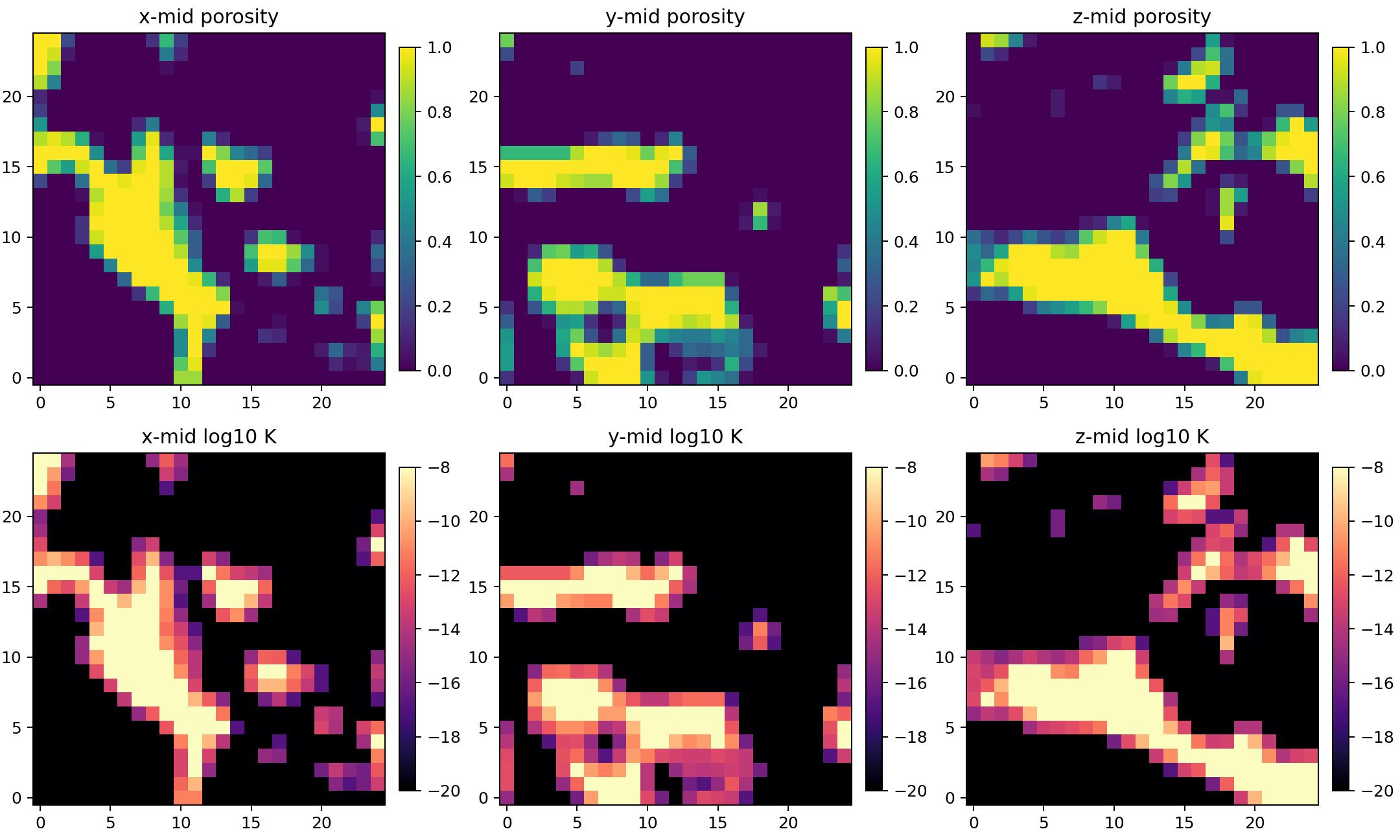
The bright connected high-porosity blocks in these midplanes explain why pure Darcy-Darcy map solves can become extremely permeable when the cap \(k_{\max}=10^{-8}\,\mathrm{m^2}\) is used.

Methods

All methods used the same \(75^3\) binary ROI or the \(25^3\) porosity/permeability map derived from that ROI.

Method label	Input	Equation or model	Discretization/backend
Direct-image LBM DNS (XLB, Stokes-limit preset)	Binary image	Low-Mach, low-Reynolds lattice-Boltzmann creeping-flow estimate	XLB/JAX adapter, 12-cell inlet/outlet buffers
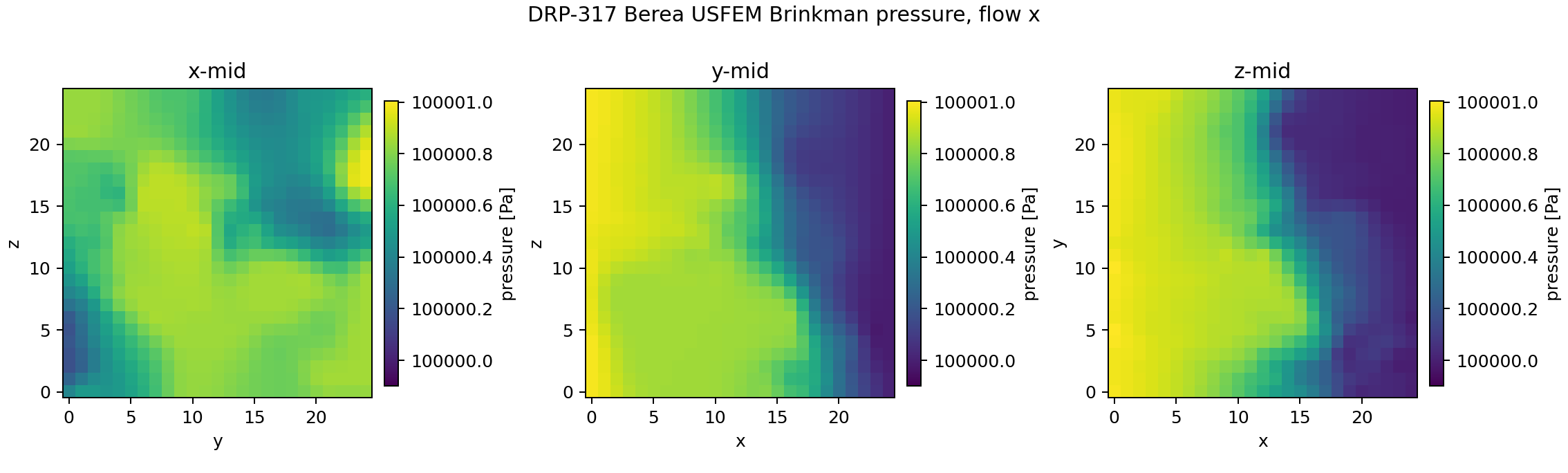
Darcy-Brinkman micro-continuum USFEM CG1 x DG1	\(\phi\) and \(k(\phi)\) maps	Darcy-Brinkman micro-continuum	FEniCSx, stabilized CG1 velocity and DG1 pressure, PETSc LU with SuperLU_DIST
Darcy-Brinkman coefficient-field Taylor-Hood CG2 x CG1	\(\phi\) and \(k(\phi)\) maps	Darcy-Brinkman micro-continuum	FEniCSx, CG2 velocity and CG1 pressure, PETSc LU with MUMPS
Darcy-Darcy coefficient-field Taylor-Hood CG2 x CG1	\(k(\phi)\) map	Mixed Darcy flow everywhere	FEniCSx, CG2 velocity and CG1 pressure, PETSc LU with MUMPS
TPFA finite-volume Darcy-Darcy	\(k(\phi)\) map	Cell-centered Darcy flow	TPFA, SciPy CG with PyAMG preconditioning
PoreSpy snow2	Binary image	Reduced pore-network model	generic_poiseuille, direct network solve
PREGO	Binary image	Reduced pore-network model	generic_poiseuille, direct network solve
Native maximal-ball	Binary image	Reduced pore-network model	generic_poiseuille, direct network solve

The direct-image LBM row solves the binary ROI rather than the Kozeny-Carman map. The Darcy-Darcy FEM and TPFA rows are retained as controls: they test the same permeability map without the Brinkman viscous term and should not be read as calibrated predictors for this cap choice.

For the direct-image LBM runs, all three directions converged under the configured steady-state criterion. The maximum lattice Mach number remained below \(3 \times 10^{-4}\), and the maximum voxel Reynolds diagnostic remained below \(1.7 \times 10^{-3}\).

The LBM row uses the package-recommended Stokes-limit preset selected in the DRP-317 LBM default sensitivity study: 12-cell inlet/outlet reservoirs, max_steps=8000, min_steps=1200, and steady_rtol=1e-4.

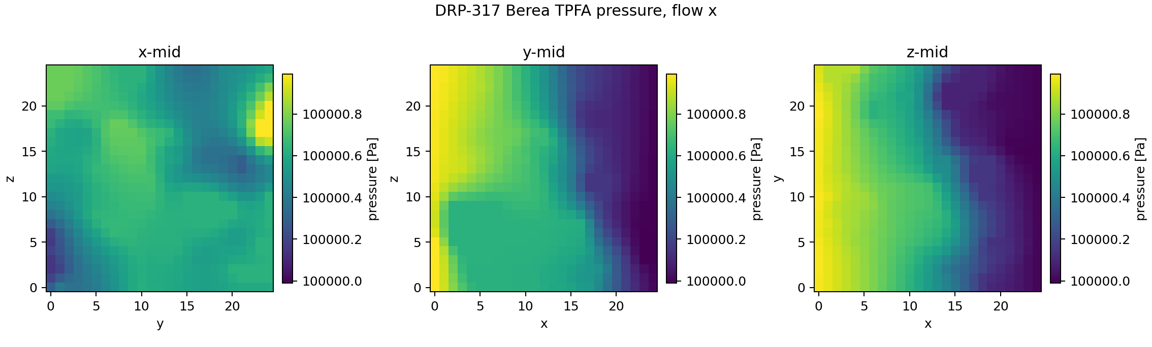
Field Outputs

The notebook also writes pressure and velocity field diagnostics for the volumetric methods. TPFA and LBM velocity fields are exported as VTU files on their regular grids. FEM pressure and velocity fields are exported as XDMF/HDF5 files after interpolation to first-order visualization spaces so they can be opened directly in ParaView.

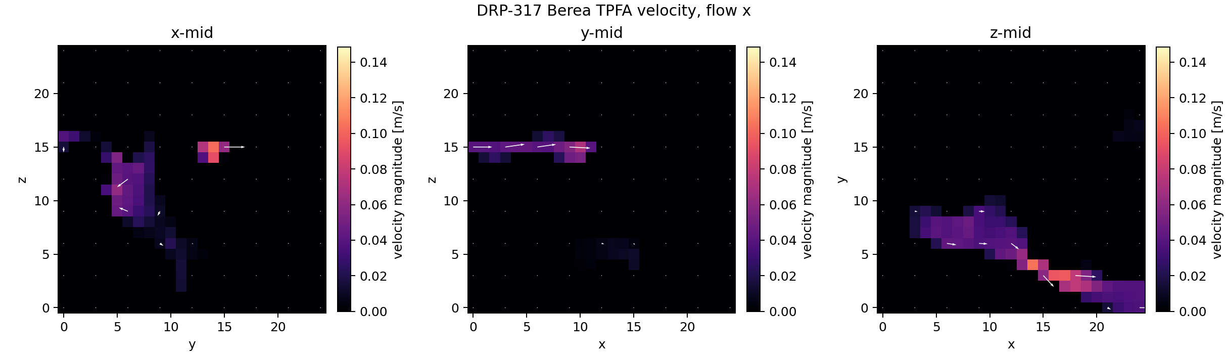
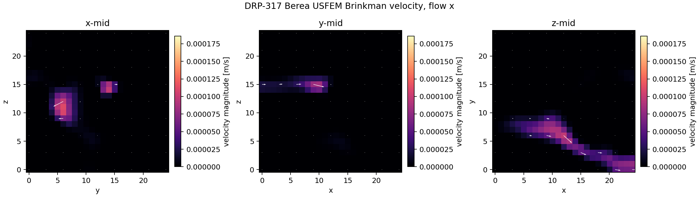
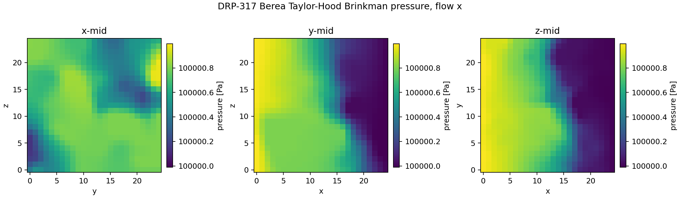
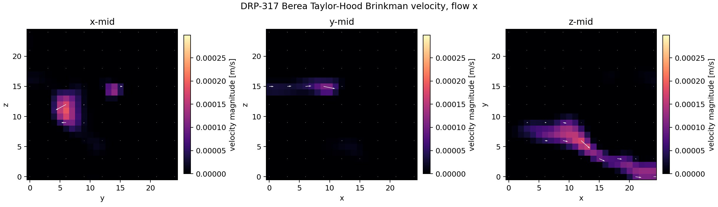
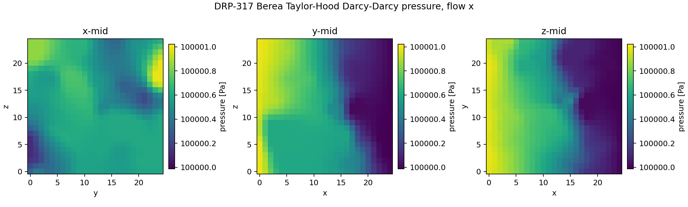
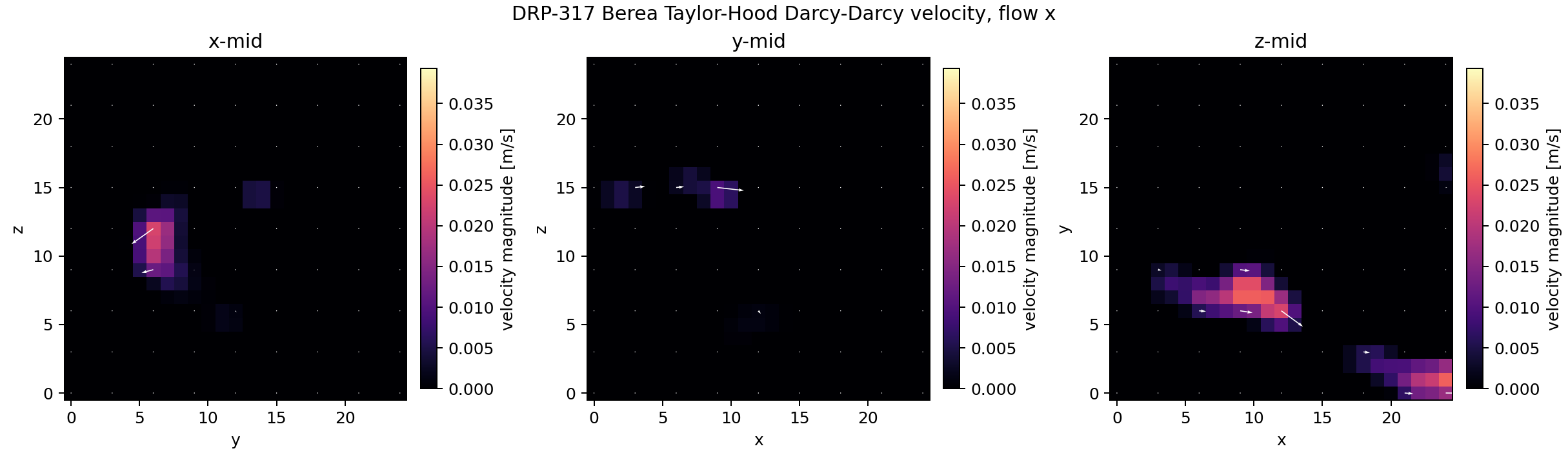
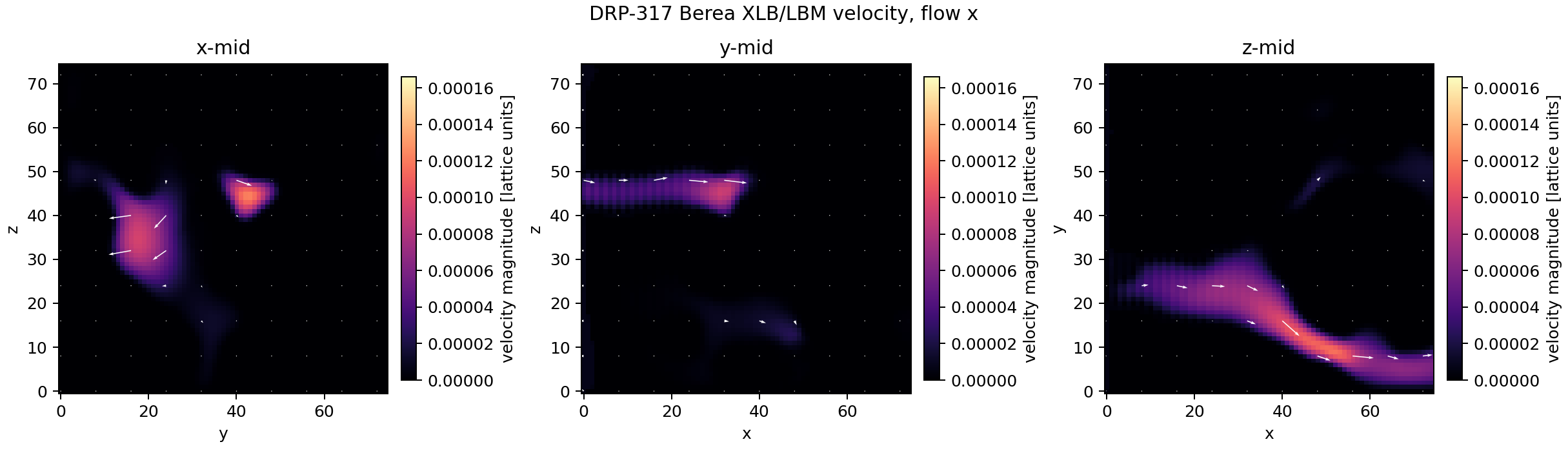
The ParaView files contain the raw solver fields. The mid-slice pressure PNGs apply only an additive pressure-gauge shift for plotting: the mean outlet-layer pressure is set to \(10^5\) Pa, while the imposed pressure drop remains \(\Delta p=1\) Pa. Therefore the pressure panels should show values near \(10^5\) Pa and variations of order 1 Pa. This shift does not change pressure gradients, fluxes, or permeability. The velocity PNGs use the raw solver scale: TPFA and FEM velocities are plotted in m/s, while the LBM velocity is plotted in lattice units because this validation workflow exports the raw lattice field. Within each PNG, the midplane panels share one color scale computed from the full plotted 3-D field.

Interpreting quiver slices

Each quiver panel can only draw the two velocity components lying in that slice. If the dominant velocity component is normal to the plane, the arrow overlay may be weak even when the velocity-magnitude color map is nonzero.

The gallery below shows the \(x\)-direction flow solve for the volumetric methods. The field-output manifest linked at the end of the page lists the corresponding files for \(x\), \(y\), and \(z\).

TPFA Darcy-Darcy

USFEM Brinkman

Taylor-Hood Brinkman

Taylor-Hood Darcy-Darcy

Direct-Image LBM

The LBM row exports a velocity field on the binary-image grid. It does not write a continuum pressure field in this validation workflow.

Pore-network models are graph-valued reductions of the image and therefore do not produce a voxel- or element-based volumetric pressure/velocity field in this study.

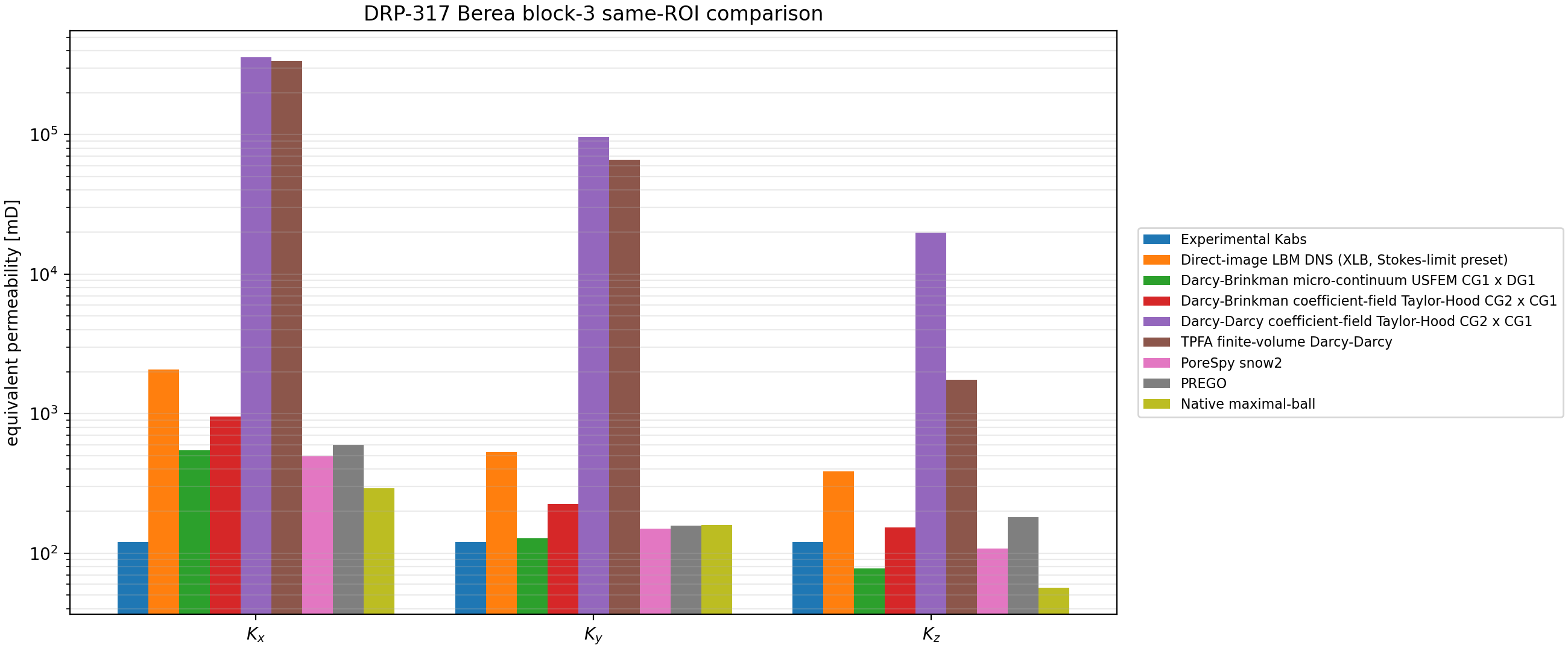
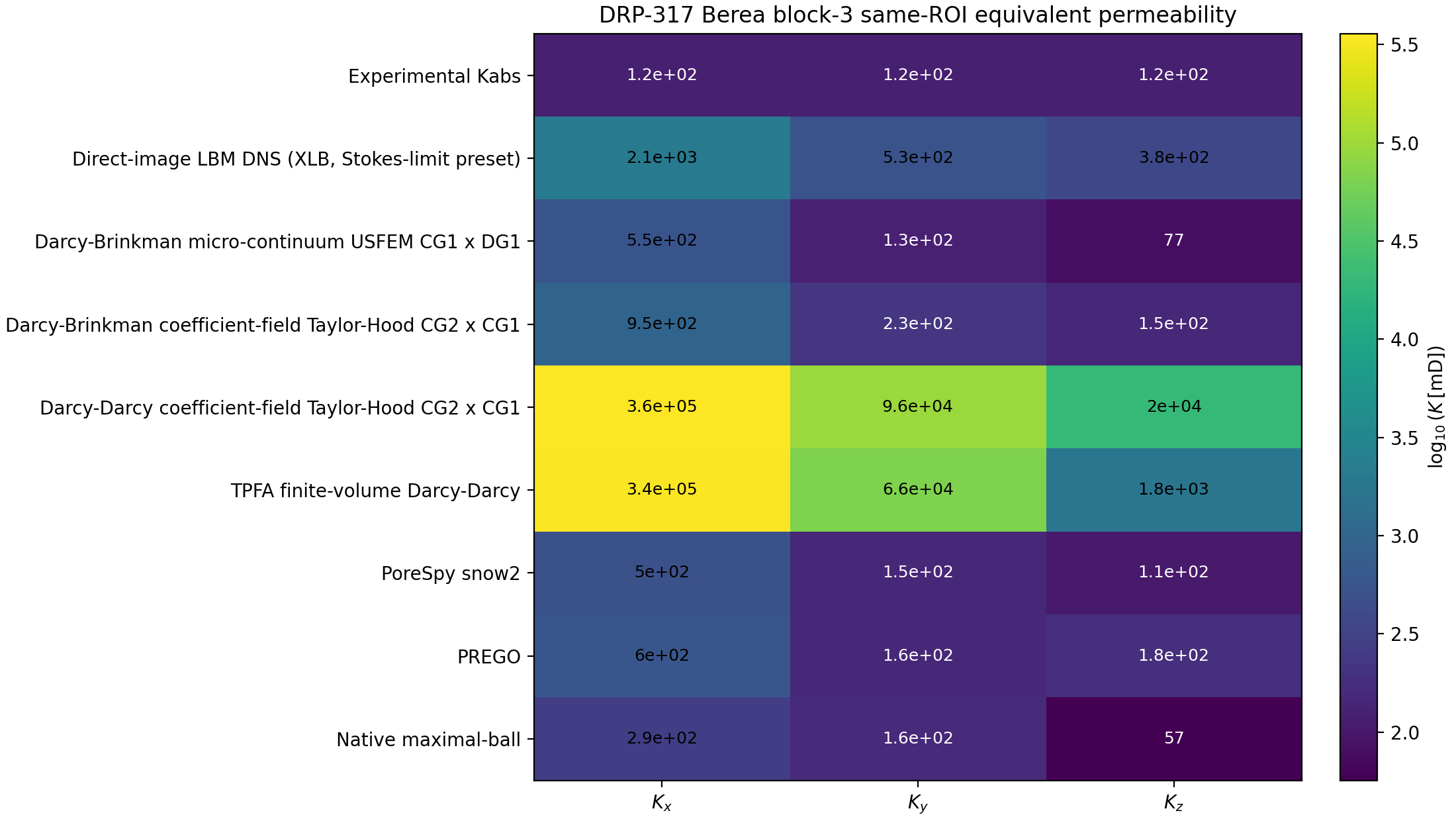
Permeability Results

The published experimental permeability for Berea is \(121.0\) mD. The table below assigns this scalar reference to \(K_x\), \(K_y\), and \(K_z\) only to make the directional simulation results visually comparable.

Method	Solver/backend	\(K_x\) [mD]	\(K_y\) [mD]	\(K_z\) [mD]
Experimental Kabs	-	121.0	121.0	121.0
Direct-image LBM DNS (XLB, Stokes-limit preset)	xlb:jax	2062.3	532.2	383.8
Darcy-Brinkman micro-continuum USFEM CG1 x DG1	fenicsx:petsc-lu-superlu_dist	547.7	127.7	77.5
Darcy-Brinkman coefficient-field Taylor-Hood CG2 x CG1	fenicsx:petsc-lu-mumps	953.5	225.0	152.5
Darcy-Darcy coefficient-field Taylor-Hood CG2 x CG1	fenicsx:petsc-lu-mumps	358,708	96,458	19,843
TPFA finite-volume Darcy-Darcy	cg+pyamg	336,235	66,223	1756.0
PoreSpy snow2	-	495.5	149.8	107.9
PREGO	-	599.4	157.9	181.6
Native maximal-ball	-	292.3	158.6	56.7

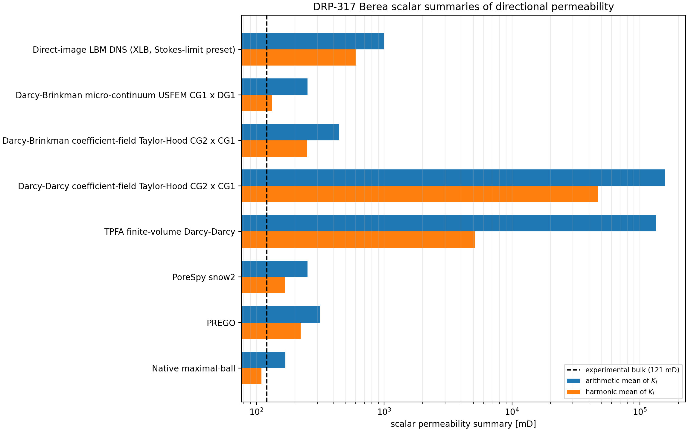
Bulk Scalar Summaries

The experimental value is reported as a scalar bulk permeability. For the directional simulations, the table and plot below summarize \(K_x\), \(K_y\), and \(K_z\) with both arithmetic and harmonic means:

\[ K_\mathrm{arith} = \frac{K_x + K_y + K_z}{3}, \qquad K_\mathrm{harm} = \frac{3}{1/K_x + 1/K_y + 1/K_z}. \]

These are scalar summaries of an anisotropic small ROI, not a substitute for the directional permeability tensor. The harmonic mean is more sensitive to the least permeable direction, while the arithmetic mean is more sensitive to highly permeable connected paths.

Method	Arithmetic mean [mD]	Harmonic mean [mD]	Arithmetic / exp	Harmonic / exp	Max/min directional K
Direct-image LBM DNS (XLB, Stokes-limit preset)	992.8	603.7	8.20	4.99	5.37
Darcy-Brinkman micro-continuum USFEM CG1 x DG1	250.9	133.0	2.07	1.10	7.07
Darcy-Brinkman coefficient-field Taylor-Hood CG2 x CG1	443.7	249.0	3.67	2.06	6.25
Darcy-Darcy coefficient-field Taylor-Hood CG2 x CG1	158336.3	47207.3	1308.56	390.14	18.08
TPFA finite-volume Darcy-Darcy	134738.0	5106.0	1113.54	42.20	191.48
PoreSpy snow2	251.1	167.0	2.07	1.38	4.59
PREGO	313.0	222.1	2.59	1.84	3.80
Native maximal-ball	169.2	109.7	1.40	0.91	5.15

Relative to the 121 mD scalar experimental reference:

Method	\(K_x/K_{\mathrm{exp}}\)	\(K_y/K_{\mathrm{exp}}\)	\(K_z/K_{\mathrm{exp}}\)	Mean absolute directional error [%]
Direct-image LBM DNS (XLB, Stokes-limit preset)	17.04	4.40	3.17	720.5
Darcy-Brinkman micro-continuum USFEM CG1 x DG1	4.53	1.06	0.64	131.4
Darcy-Brinkman coefficient-field Taylor-Hood CG2 x CG1	7.88	1.86	1.26	266.7
Darcy-Darcy coefficient-field Taylor-Hood CG2 x CG1	2964.53	797.17	164.00	130756.4
TPFA finite-volume Darcy-Darcy	2778.80	547.30	14.51	111253.7
PoreSpy snow2	4.10	1.24	0.89	114.7
PREGO	4.95	1.30	1.50	158.6
Native maximal-ball	2.42	1.31	0.47	75.2

Performance

The table reports the solver wall times recorded by the notebook for this local run. These timings are useful for comparing methods within the same machine and software stack, but they are not portable benchmark guarantees.

Method	Mean time per direction [s]	Total 3-axis time [s]	Total 3-axis time [min]
Direct-image LBM DNS (XLB, Stokes-limit preset)	107.3	321.9	5.36
Darcy-Brinkman micro-continuum USFEM CG1 x DG1	151.7	455.2	7.59
Darcy-Brinkman coefficient-field Taylor-Hood CG2 x CG1	166.2	498.7	8.31
Darcy-Darcy coefficient-field Taylor-Hood CG2 x CG1	165.4	496.3	8.27
TPFA finite-volume Darcy-Darcy	0.2	0.6	0.01
PoreSpy snow2	0.7	2.0	0.03
PREGO	0.3	0.9	0.01
Native maximal-ball	0.2	0.6	0.01

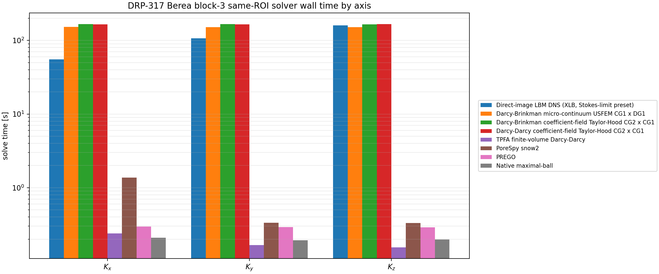
The shipped FEM rows completed the three directions in roughly eight minutes each for the \(25^3\) map on this machine. The TPFA and pore-network solves are much faster on this small problem. That runtime should not be confused with greater physical fidelity: the TPFA row is solving a different, pure Darcy coefficient-field model.

Interpretation

Several conclusions are scientifically useful:

• The same ROI is strongly anisotropic at this size. Almost every method predicts a much larger \(K_x\) than \(K_y\) or \(K_z\), including the direct-image LBM row. This suggests the \(75^3\) crop contains a preferential connected path and should not be treated as a bulk representative volume.
• The scalar-summary plot makes this anisotropy visible: arithmetic means are consistently higher than harmonic means, and the TPFA row has \(K_\mathrm{max}/K_\mathrm{min}\approx 191\). The USFEM Brinkman harmonic mean is close to the experimental scalar, but that agreement is partly caused by combining one high and two lower directional estimates.
• The Darcy-Brinkman USFEM row is the closest map-based continuum row in the \(y\) direction and gives a reasonable \(z\)-direction magnitude, but it still overpredicts \(K_x\) by a factor of about 4.5. The Taylor-Hood Brinkman row is more permeable for all three axes with the current coefficient map.
• The pure Darcy-Darcy rows produce enormous values because the Kozeny-Carman map contains connected cells at the \(10^{-8}\,\mathrm{m^2}\) cap. These rows are useful diagnostics for the coefficient map and boundary convention, but they are not validated predictors for this cap choice.
• The pore-network rows are very fast and, for \(y\) and \(z\), are in the same order of magnitude as the experimental reference. Their \(K_x\) values remain high, again consistent with an ROI-scale connected path rather than a solver-only artifact.
• The direct-image LBM row is substantially above the experimental scalar in all directions. Since it does not use the Kozeny-Carman map, this mismatch is evidence that the small binary ROI and segmentation/representativeness assumptions are central to the validation error. The separate LBM sensitivity study shows that the stricter 12-cell reservoir preset changes the LBM values by only a few percent, so the mismatch should not be explained away as a loose steady-state tolerance artifact.

The most conservative reading is that the current FEniCSx Brinkman implementations are numerically credible for this map size, while the experimental mismatch is dominated by ROI representativeness and coefficient closure rather than by the linear solvers alone. Finer maps, larger ROIs, and controlled sensitivity studies for \(d\), \(C\), \(k_{\max}\), and the experimental porosity mismatch are required before treating any single method as a calibrated predictor for the full Berea sample.

Reproducible Artifacts

• Case summary CSV
• Map summary CSV
• Model comparison CSV
• Ratios to experiment CSV
• Bulk permeability means CSV
• Direct-image LBM directional CSV
• Direct-image LBM status JSON
• Field-output manifest CSV