Two-Dimensional Brinkman MMS Report

This report verifies the three shipped mixed finite-element formulations against one known, smooth solution. It is a software-verification case: the forcing is chosen to make the prescribed fields exact. It is not evidence that a porous-medium closure is physically valid.

Strong problem and exact fields

On \(\Omega=(0,1)^2\), solve

\[ -\nu\Delta\mathbf u+\gamma\mathbf u+\nabla p=\mathbf f,\qquad \nabla\cdot\mathbf u=0, \]

with \(\nu=0.1\), \(\gamma=1\), and

\[ g(s)=s-\frac{\exp((s-1)/\nu)-\exp(-1/\nu)} {1-\exp(-1/\nu)},\qquad \mathbf u_{\rm ex}=(g(y),g(x)),\qquad p_{\rm ex}=x-y. \]

Because the first velocity component depends only on \(y\) and the second only on \(x\), \(\nabla\cdot\mathbf u_{\rm ex}=0\) exactly. voids constructs

\[ \mathbf f=-\nu\Delta\mathbf u_{\rm ex} +\gamma\mathbf u_{\rm ex}+\nabla p_{\rm ex} \]

as a UFL expression. The complete-boundary condition is \(\mathbf u=\mathbf u_{\rm ex}\) on \(\partial\Omega\). Pressure has no physical point gauge; before measuring its error, the mean of \(p_h-p_{\rm ex}\) is removed.

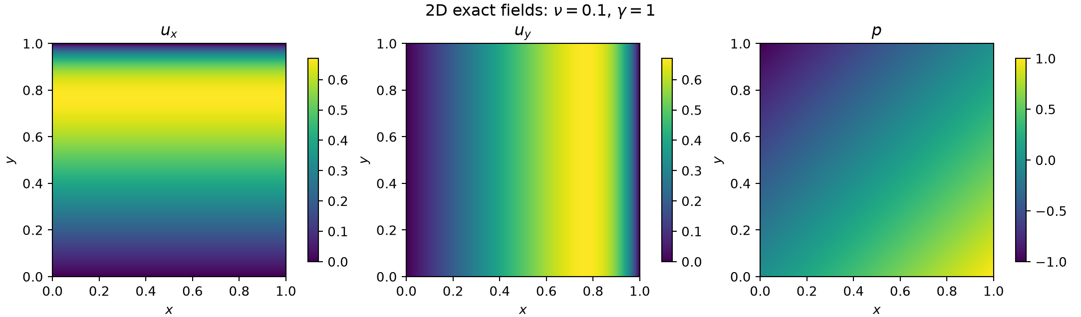
The exponential layers at \(x=1\) and \(y=1\) test whether the mesh sequence has reached the asymptotic range. The gentler \(\nu=0.1\) case is used here so that all five meshes resolve the layer; the reference \(\nu=0.01\) case needs a substantially finer terminal mesh.

Discretizations and measured errors

The study compares Taylor--Hood \([\mathrm{CG}_2]^2\times\mathrm{CG}_1\), USFEM \([\mathrm{CG}_1]^2\times\mathrm{DG}_0\), and USFEM \([\mathrm{CG}_1]^2\times\mathrm{DG}_1\). The USFEM runs use physical interior-edge length (facet_size_mode="facet_diameter"). Errors are

\[ e_u^{L^2}=\|\mathbf u_{\rm ex}-\mathbf u_h\|_{L^2},\quad e_u^{H^1}=\|\mathbf u_{\rm ex}-\mathbf u_h\|_{H^1},\quad e_p^{L^2}=\|p_{\rm ex}-p_h-c_h\|_{L^2}. \]

The five structured triangulations have \(n=(4,8,16,32,64)\), \(h=1/n\), and \((32,128,512,2048,8192)\) cells. Every marker below is one completed solve. Each right triangle uses the two finest \(h\) values; its annotation is the measured slope \(r=\log(e_{i-1}/e_i)/\log(h_{i-1}/h_i)\), not an imposed guide line.

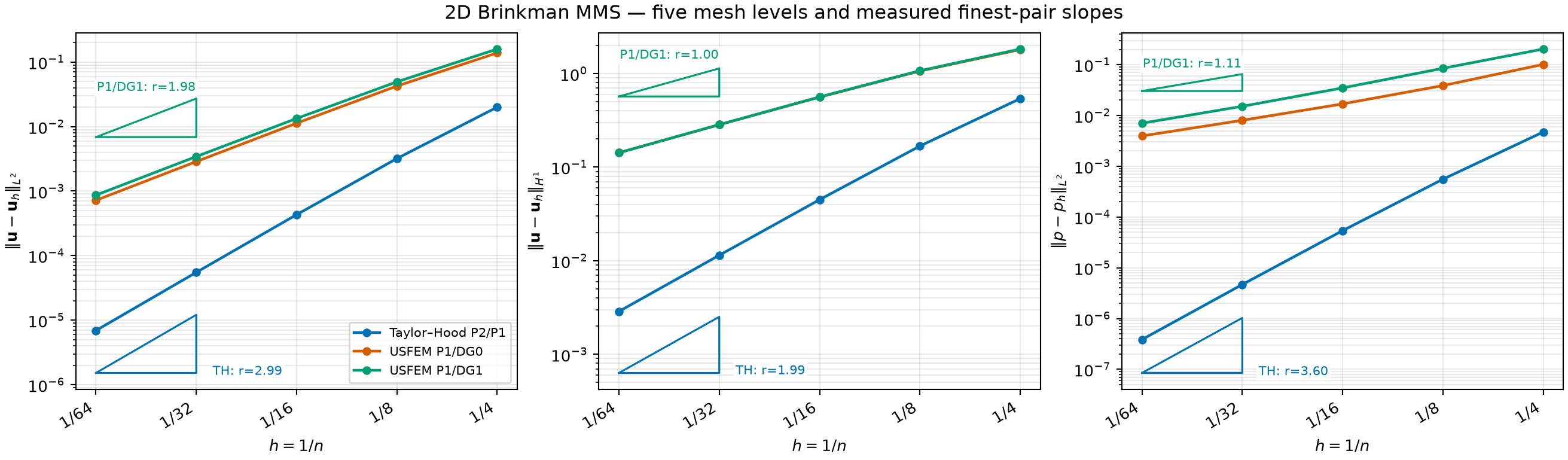
Method	\(r(L^2_u)\)	\(r(H^1_u)\)	\(r(L^2_p)\)	Finest \(L^2_u\)	Finest \(L^2_p\)
Taylor--Hood P2/P1	2.992	1.993	3.600	\(6.924\,10^{-6}\)	\(3.858\,10^{-7}\)
USFEM P1/DG0	1.994	0.995	1.024	\(7.199\,10^{-4}\)	\(3.944\,10^{-3}\)
USFEM P1/DG1	1.985	0.997	1.107	\(8.668\,10^{-4}\)	\(7.030\,10^{-3}\)

The velocity orders recover the nominal \(3/2\) Taylor--Hood and \(2/1\) linear-element behavior. Both USFEM pressure rates recover first order. Taylor--Hood pressure is superconvergent for this mesh/case pairing; that observed \(3.60\) must not be generalized into a nominal P1-pressure theorem. The complete machine-readable table is available as CSV.

Executable MWE

The full script is examples/fem_mms/mms_2d.py. It performs all 15 solves, asserts the rate thresholds, writes the CSV, and recreates both figures:

pixi run python examples/fem_mms/mms_2d.py \
  --output-dir examples/outputs/fem_mms/2d

Change viscosity, reaction, mesh sequence, and solver options near the top of main. A rate failure on a deliberately coarse or sharp-layer sequence is a diagnostic to refine the mesh, not by itself proof of a formulation defect.