Three-Dimensional Body-Fitted Vug Verification

This page documents a body-fitted spherical FEM benchmark for pressure, velocity, and flow-based upscaling. It has no known exact flow solution, so it is a synthetic verification benchmark rather than MMS.

Body-fitted FEM flow benchmark

The spherical benchmark and its volume-fraction sweep are the 3D counterparts of the 2D body-fitted family. Its role is formulation parity, flow-based upscaling, geometry/provenance checking, and report-value regression.

Geometry and coefficients

The unit cube contains a centered sphere of radius \(r=0.25\). Its analytic volume fraction is

\[ f_v=\frac{4\pi r^3}{3}=0.0654498. \]

The nondimensional benchmark uses \(\nu=10^{-2}\), \(\gamma_m=10^7\), \(\gamma_v=1\), \(p_L=1\), and \(p_R=-1\). Natural pressure traction acts at \(x=0,1\); the four transverse walls impose zero normal velocity. Gmsh fragments the cube and sphere and transfers physical volume, exterior, and interface tags.

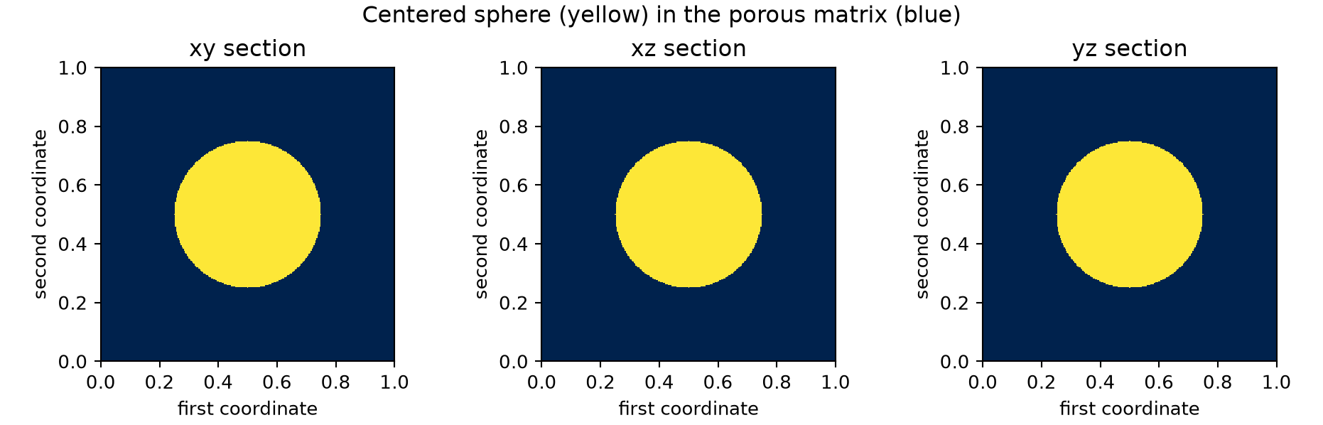
Formulation comparison and field sections

The gallery compares Taylor--Hood P2/P1 with P1/DG1 USFEM on the same body-fitted mesh. The USFEM branch uses the shifted 3D facet law and facet_size_mode="facet_measure", namely \(\sqrt{|F|}\) for a triangular facet. That is a measure-based length, not an exact diameter for an arbitrary triangle.

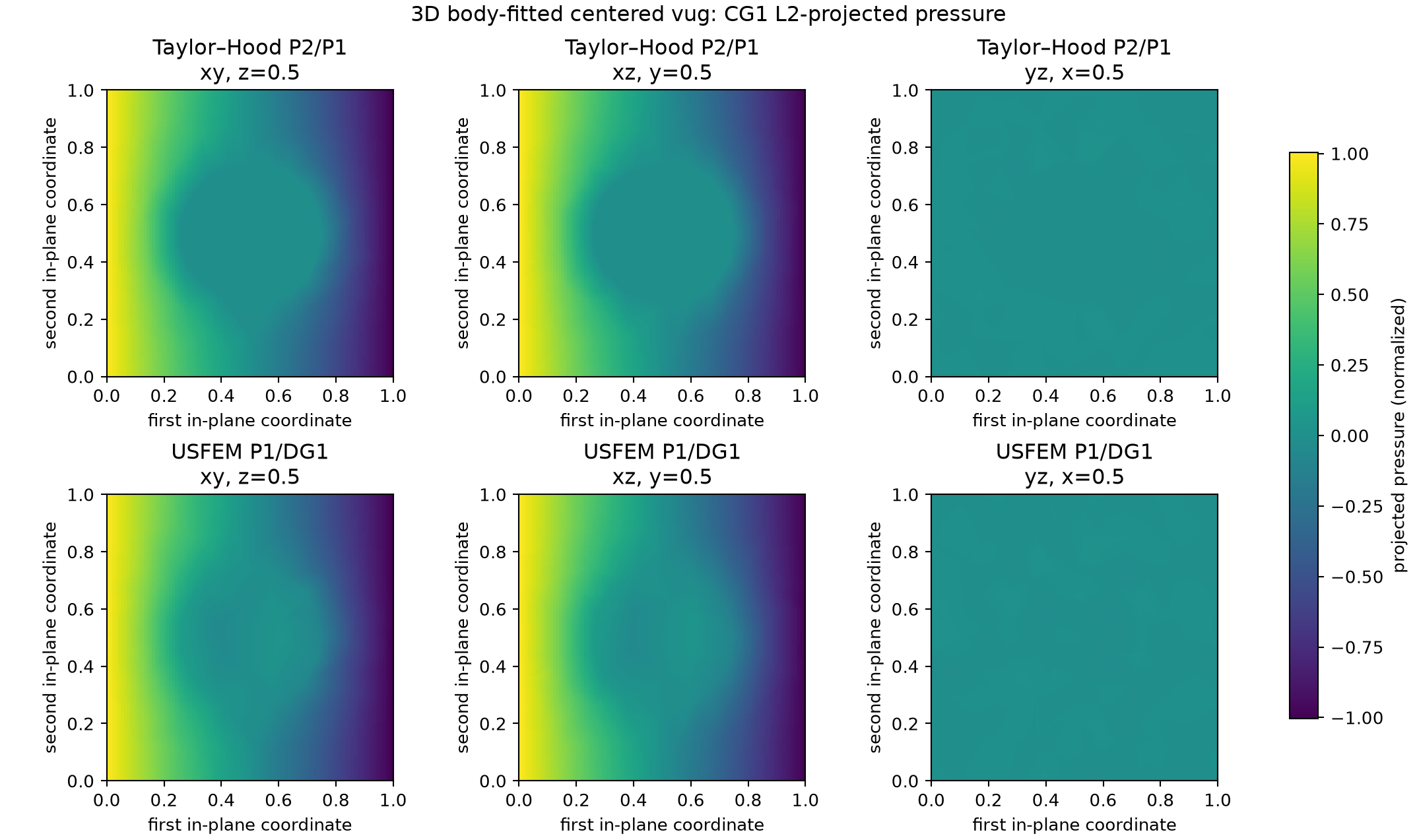
Taylor--Hood pressure is continuous, whereas the USFEM pressure space is \(\mathrm{DG}_1\). For the comparison above, each raw pressure is projected onto continuous CG1 by the \(L^2\) problem

\[ (\widetilde p_h,w_h)=(p_h,w_h) \qquad\forall w_h\in\mathrm{CG}_1. \]

This changes only the visualization field: flux, permeability, and the reported solve all use the unmodified discrete pressure. The raw DG1 result is shown below as a diagnostic; its triangular element-to-element jumps are an expected property of the discontinuous pressure space and must not be hidden or mistaken for the projected field.

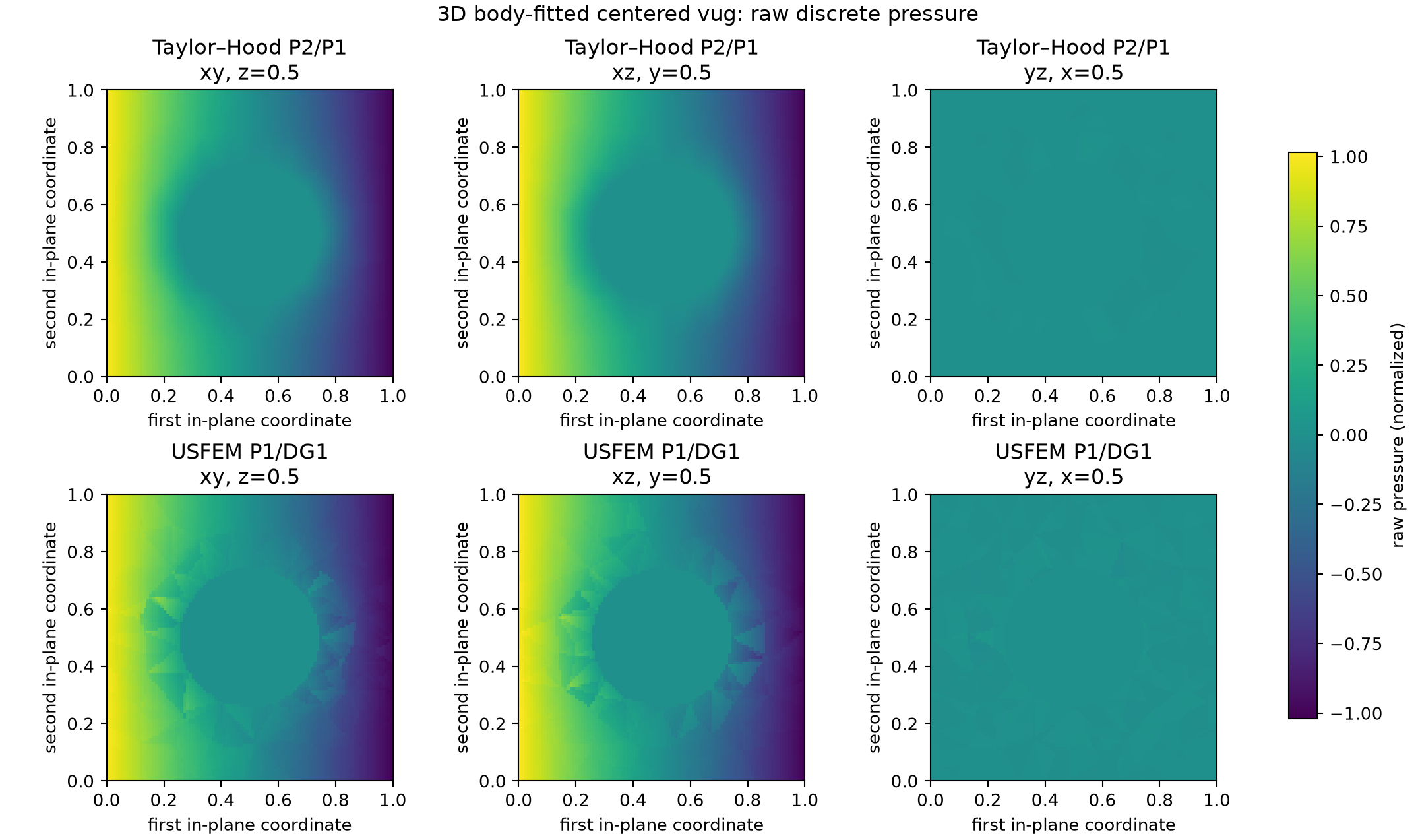
A focused P1/DG1 refinement check gives:

Nominal resolution	Tetrahedra	\(\|[p_h]\|_{L^2(\mathcal F_h)}\)	Outlet flux
8	834	0.37295	\(2.24249\,10^{-7}\)
12	1,968	0.33548	\(2.31423\,10^{-7}\)
16	5,018	0.22761	\(2.37442\,10^{-7}\)

The raw jump diagnostic decreases with refinement while the flux approaches the report-scale value. This supports the interpretation that the faceting is a coarse-mesh DG visualization effect, rather than evidence that a continuous pressure was assembled incorrectly. The three meshes are not a sufficient asymptotic sequence for assigning a jump-convergence rate.

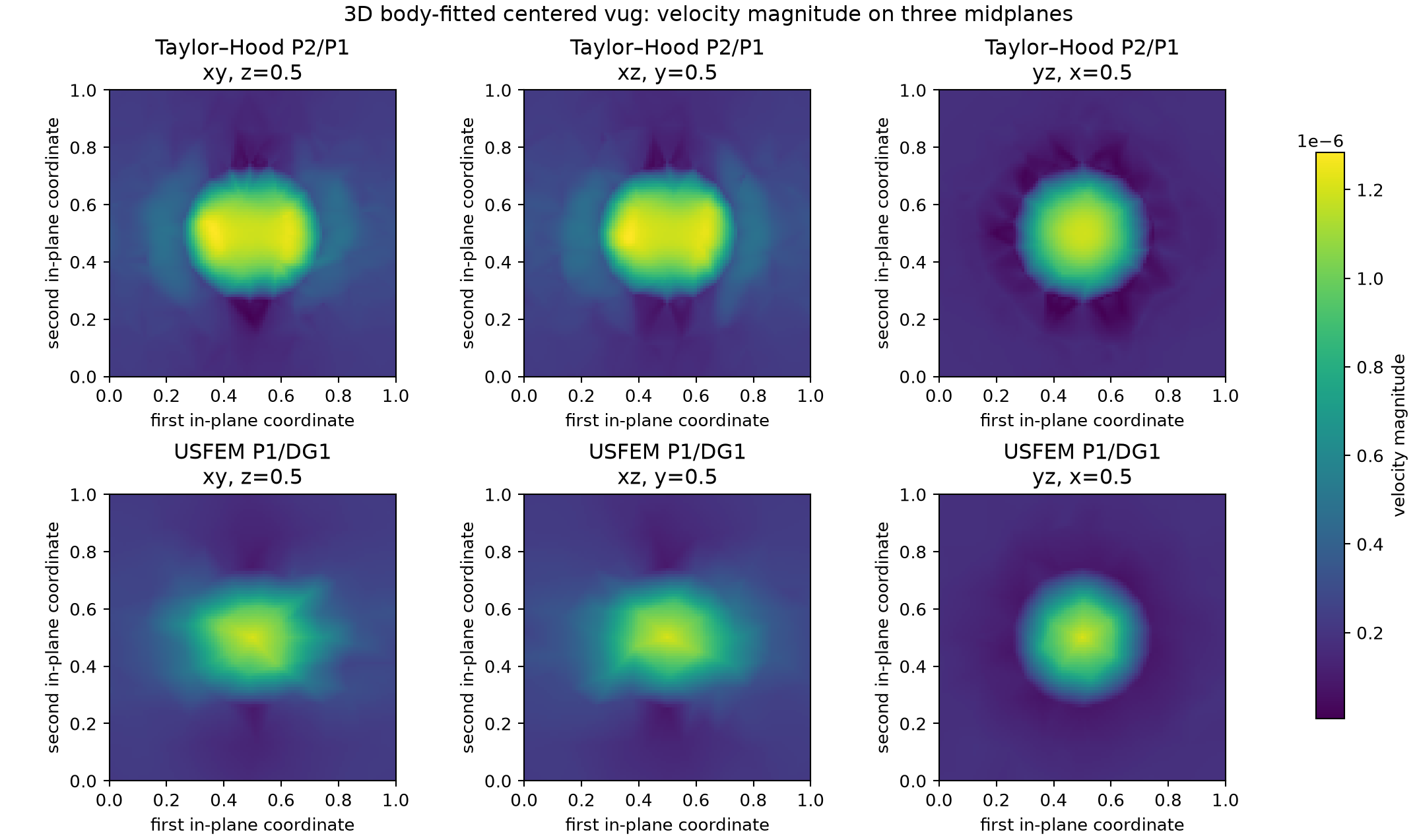
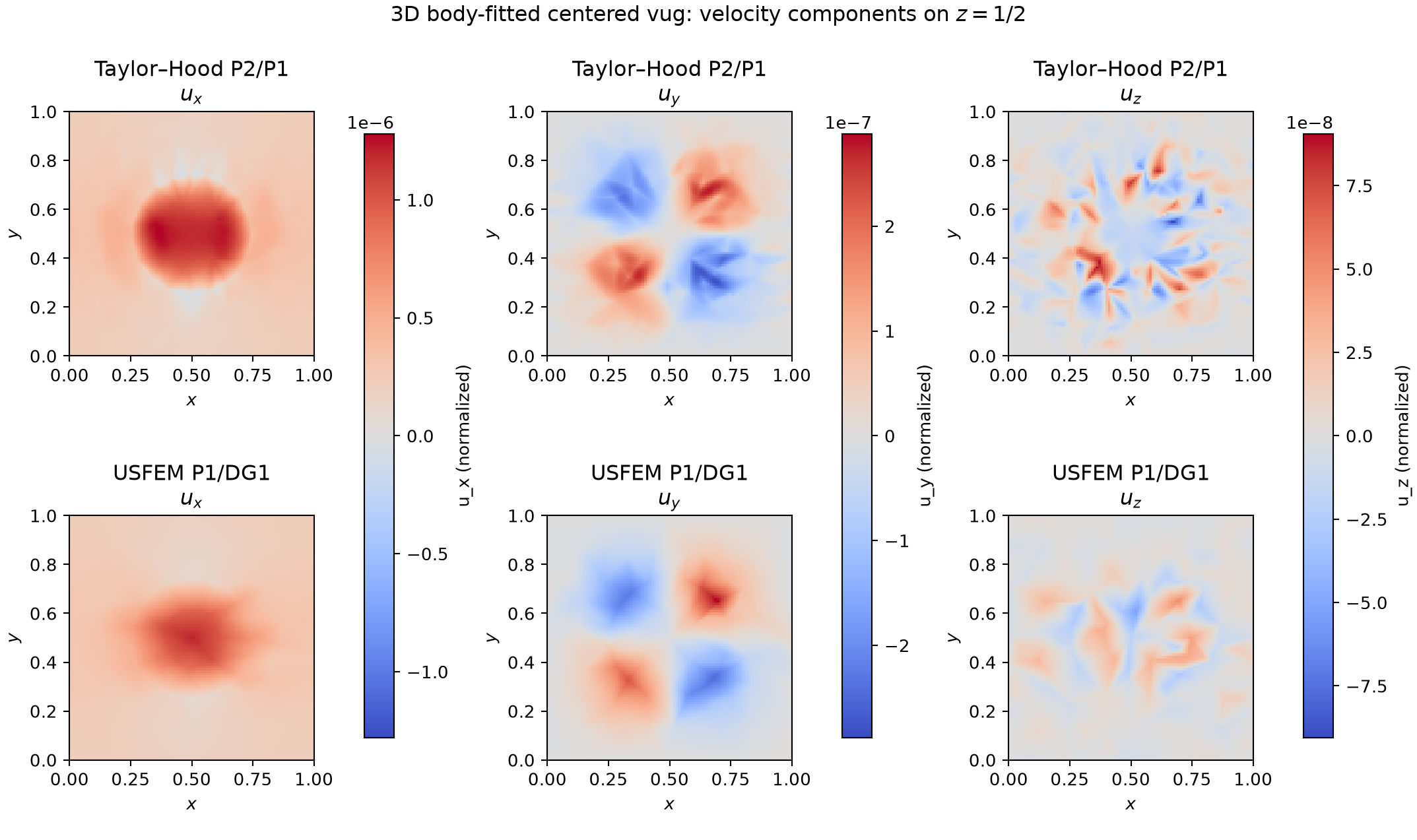
Pressure is shifted to zero volume mean only after the solve. Each pressure gallery uses common color limits across methods. These resolution-16 sections are a qualitative field and implementation audit, not the report-scale flux result. The exact cell count, represented fraction, flux, and timings are available as CSV.

Resolution-16 method	Tetrahedra	Represented \(f_v\)	Outlet flux
Taylor--Hood P2/P1	5,018	0.06193	\(2.42981\,10^{-7}\)
USFEM P1/DG1	5,018	0.06193	\(2.37442\,10^{-7}\)

The USFEM/Taylor--Hood flux ratio is \(0.9772\). The remaining 2.28% mismatch, and the visible local field differences, are reasons to retain the finer report profile rather than declaring mesh convergence from this gallery.

Flow-based upscaling

For a cube of length \(L\), outlet area \(A=L^2\), and imposed pressure drop \(\Delta p\), the flow-based permeability is

\[ K_{\rm eff}=\frac{\mu L\,Q}{A\,\Delta p}. \]

The nondimensional benchmark has \(L=A=1\), \(\Delta p=2\), and matrix permeability

\[ K_m=\frac{\nu}{\gamma_m}=10^{-9}. \]

The study converts each requested spherical volume fraction to

\[ r=\left(\frac{3f_v}{4\pi}\right)^{1/3} \]

and solves both formulations on independently regenerated but deterministic body-fitted meshes. A centered sphere must satisfy \(f_v<\pi/6\approx0.524\) to remain inside the cube. The family therefore uses

\[ f_v\in\{0,\ 0.01,\ 0.05,\ 0.10,\ 0.20,\ 0.30,\ 0.40\}; \]

using the 2D values 0.6 or 0.7 would require a different, clipped, or superellipsoidal inclusion.

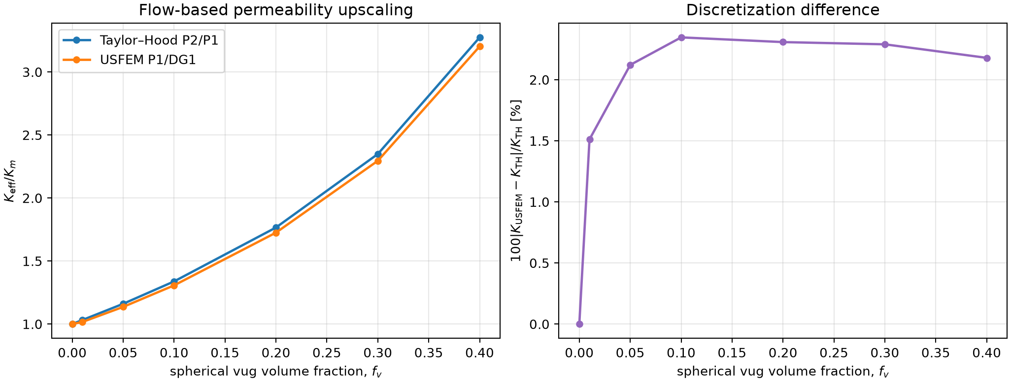
The right panel is a discretization comparison, not a difference between two constitutive models:

\[ \delta_K= 100\frac{\left|K_{\rm USFEM}-K_{\rm TH}\right|}{K_{\rm TH}}. \]

Both branches solve the same piecewise Darcy--Brinkman equations and use the same coefficients and boundary conditions.

Analytic \(f_v\)	Represented \(f_v\)	\(K_{\rm eff}/K_m\), Taylor--Hood	\(K_{\rm eff}/K_m\), USFEM	\(\delta_K\) [%]
0.00	0.00000	1.0000	1.0000	\(<10^{-6}\)
0.01	0.00828	1.0320	1.0164	1.5115
0.05	0.04657	1.1606	1.1360	2.1210
0.10	0.09564	1.3383	1.3069	2.3463
0.20	0.19430	1.7658	1.7250	2.3077
0.30	0.29374	2.3488	2.2950	2.2895
0.40	0.39280	3.2742	3.2029	2.1787

These curves use nominal resolution 16. Linear tetrahedra under-represent the curved sphere, especially for the smallest inclusion. The complete upscaling CSV therefore records both analytic and represented fractions rather than silently equating them.

A focused \(f_v=0.40\) mesh check gives:

Resolution	Tetrahedra	Represented \(f_v\)	Taylor--Hood \(K_{\rm eff}/K_m\)	USFEM \(K_{\rm eff}/K_m\)	\(\delta_K\) [%]
8	1,095	0.37258	3.1353	2.9208	6.8421
16	5,409	0.39280	3.2742	3.2029	2.1787
24	14,115	0.39644	3.2750	3.2409	1.0413

The Taylor--Hood endpoint changes by only 0.025% from resolution 16 to 24, whereas the USFEM endpoint changes by 1.18%. The method difference also continues to decrease. Thus the monotone upscaling trend is established, but the resolution-16 USFEM curve must not be presented as fully mesh-converged.

The report regression profiles use target mesh size \(\sqrt3/30\): 3d_centered_vug_p1dg1 targets \(Q_R=2.413\,10^{-7}\), and 3d_centered_vug_taylor_hood targets \(Q_R=2.42167\,10^{-7}\), with 1% flux tolerance and 3% represented-volume tolerance. Those are numerical reference targets, not experimental validation.

Executable MWE

examples/fem_mms/vug_3d.py recreates the seven-fraction upscaling study, both field solves, all 12 pressure/velocity midplane panels, the component gallery, and both summaries:

pixi run python examples/fem_mms/vug_3d.py

Use --skip-fields to run only the upscaling sweep, or --skip-upscaling to regenerate only the field galleries. The sweep is configurable, for example:

pixi run python examples/fem_mms/vug_3d.py \
  --skip-fields \
  --upscaling-resolution 24 \
  --upscaling-fractions 0 0.01 0.05 0.1 0.2 0.3 0.4

Add --export-xdmf to write the representative velocity/pressure results for ParaView. Convergence of an integral quantity must not be inferred from a visually smooth coarse field.